2. Mapping Tutorial • SMARTR

0 Pre-processing

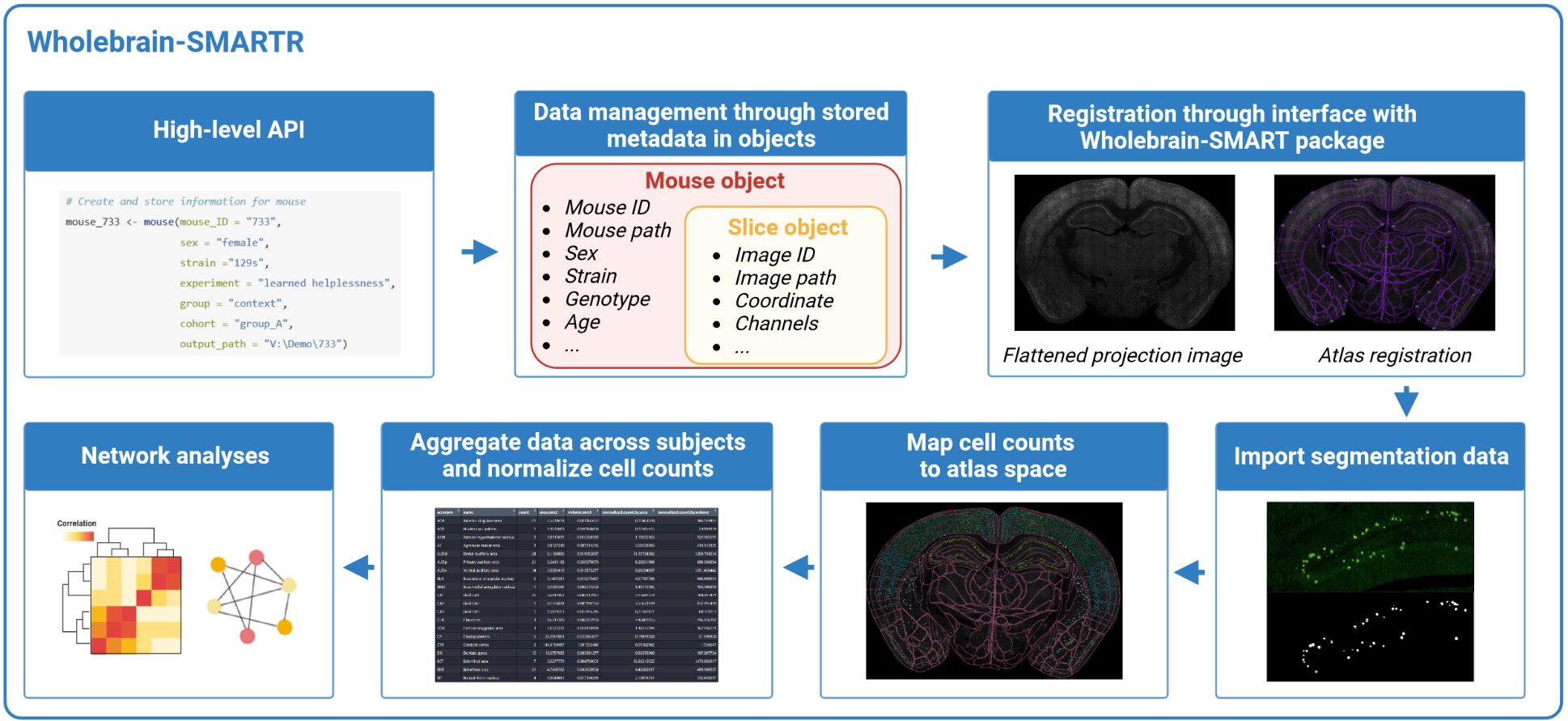
SMARTR encapsulates the process of registration, importation of segmentation data, and performs downstream analysis. Prior to this, the imaging data must be pre-processed and cells are separately segmented in ImageJ/FIJI. We have a separate, in-depth article on our imaging approach, parameters, and segmentation process. We suggest starting there if you would like to walk through the pipeline from raw example image. The remainder of this page will focus on steps relevant to registration, segmentation data import, and downstream data analysis using SMARTR. We recommend completing the pre-processing and segmentation tutorial with the example image so you can walk through the SMARTR tutorial with this data.

0.1 File organization

Each image file is stored in a hierarchical folder structure in a slice folder then a mouse folder:

Root folder > project folder > ... > mouse no. > slice name > image file

The image files, which we also refer to as slices, are assumed to follow the naming convention mouseNo_slice.ext.

The slice is a unique tag or index used to identify the particular section when it was imaged. For example, we use an indexing system where the first number identifies the slide number and a second number identifies position on that slide. These numbers are separated by an underscore. Therefore the slice 1_1 represents section one of slide one for this animal. Of course, other indexing approaches can be used. We create a slice name by concatenating the slice with the mouse ID separate by an underscore to name images unambiguously.

For example, here is one of our image directory paths:

V:/Learned_Helplessness/Mapping_Images/Shock/733/733_1_1

And this is the file path to the image stored in that directory:

V:/Learned_Helplessness/Mapping_Images/Shock/733/733_1_1/733_1_1.lif

Here, the image or slice name is 733_1_1.lif with the slice no. being 1_1. This section came from mouse 733. This heirarchical file structure is helpful, as all segmentation files and pre-processing files will be stored in each image folder while all mouse object files will be stored in the parent mouse directory.

0.2 Flatten any z-stacks for registration

Although cell counts may be segmented in 3D, during the registration process, a single coronal atlas plate from the Allen Mouse Brain Atlas is fitted to a 2D .tif image. Therefore, if you are processing any z-stack images, they need to be flattened and channels need to be collapsed into a single image used for the purpose of registration. This step needs to be completed prior to using SMARTR for registration. We detail how to do this in using our pre-processing article

1 Tutorial outline

In this tutorial, We will walk through the following steps using an example preprocessed image:

Setting up the pipeline by specifying experimental parameters and save directories.
The interactive registration process.
Importing raw segmentation data from .txt files generated from ImageJ for multiple channels. This data will then be transformed into a segmentation object that is compatible with wholebrain functions.
Combining the segmentation and registration data to map cell counts onto a standardized mouse atlas. VI Cleaning the mapped data in all the following ways:
1. Removing cells that map outside the boundaries of the atlas.
2. Omitting regions by a default list of regions to omit.
3. Omitting new regions to omit by user-curated list for each image.
4. Removing cells from a contralateral hemisphere per slice if the registrations are divided by right and left hemispheres.
Obtaining cell counts normalized by region volume (per mm³) and region areas (per mm²).
(Optional) Splitting the hippocampal cell counts into dorsal and ventral based on a user-defined AP coordinate ranges. IX Aggregating cell counts across multiple animals.
Quality checks to look for outliers in region cell counts prior to analysis.
Functions for easy analysis, based on categorical variables entered as mouse attributes. These will include functions for region cross correlations and network analyses.

Functions for analysis and automated visualization are detailed in our example analysis notebook

These steps will be achieved through functions that operate on objects in SMARTR. Objects are used to store raw data and processed data, as well as imaging, animal, and experimental parameters relevant to the analysis. Note that in a separate article, we describe ways to scale-up many of these steps to map images in a high-throughput manner with scripts. The modularity of these functions lend to the creation of many different custom workflows. We provide links to example notebooks that others can modify for their own datasets.

2 Pipeline setup

Okay, let’s walkthrough the pipeline with an example mouse and image to process!

# Load SMARTR
library(SMARTR)

You can download our example fully pre-processed image folder here. This image came from mouse 733, so create a empty folder named 733 in a location of your choice and upzip the image folder into this folder.

2.1 Initializing a mouse object

Let’s create an instance of a mouse object. This mouse object will store data from mouse No. 733, so we will name it mouse_733. We also want to store the important experiment metadata related to this mouse. All of this can be done using the SMARTR::mouse() constructor function:


# Create and store information for mouse 
mouse_733 <- mouse(mouse_ID = "733",
                   sex = "female",
                   strain ="129s",
                   experiment = "learned helplessness",
                   group = "context",   # Flexible attribute to encapsulate different experimental conditions, e.g. genotype, behavior conditions, that doesn't fit into other categories.
                   cohort = "group_A",
                   output_path = "V:/Michelle_Jin/Wholebrain pipeline/733")   # replace the output path with the path to your specific mouse folder
            

print(mouse_733)

Note that when we don’t initially store the mouse metadata using variables passed to the mouse object constructor, this metadata is ‘empty’ and there are default values stored as placeholders.

print(mouse())

2.2 Modifying mouse attributes

If you find that you’ve made a mistake in setting the attributes for a mouse object, don’t worry. These attributes can be easily modified. We just need to pull out the info list containing the mouse attributes and manually correct them:

# get the mouse info list
mouse_info <- attr(mouse_733, 'info')

# Change mouse attributes to reflect your mouse and experiment.
mouse_info$sex           <- 'male'
mouse_info$group         <- 'shock'
mouse_info$cohort        <- "group_B"

# Change mouse's attributes by storing the mouse info list back into the mouse
attr(mouse_733, 'info') <- mouse_info

# Check the updates 
print(mouse_733)

We have now finished setting up a mouse object and are ready to store some imaging and automated cell count data into it!

2.3 Initializing a slice object

Now we need to create a slice object. We also want to store imaging metadata as the slice object’s attributes. For this we’ll use the SMARTR::slice() constructor function.

Before doing this, look at your image and compare it with a standardized mouse atlas to decide what the most accurate AP coordinate should be prior to creating the object. You can reference either the SMART reference atlas or http://openbrainmap.org. In our example image, we’ve already pre-assigned the coordinate.

Additionally, if you need to process each hemisphere separately due to hemisphere separation, tears, etc, it should be specified. There are built-in ways to clean data from a right hemisphere slice and omit the contralateral hemisphere for demonstration. If the left and right side align well onto a single atlas plate, initialize only one slice object and set the hemisphere attribute to NULL (or don’t set it, as this is the default).

s <- slice(slice_ID = "1_4",  
           coordinate = -2.14,         # AP coordinate that matches best matches the images
           conversion_factor = 1.0833, # Pixel-to-micron conversion factor. 
           bin = 1,                    # If the image was downsampled by a bin factor in imageJ
           z_width = 9,                # z-stack thickness in microns
           hemisphere = NULL,          # "left", "right" or NULL (both sides). This is necessary if you are only processing one hemisphere due to hemisphere separation, tears, etc.
           channels = c('cfos', 'eyfp', 'colabel'),  # Channels to process
           # registration_path = 'V:/Michelle_Jin/Wholebrain pipeline/733/733_1_4/MAX_733_1_4.tif'# Path to the registration image. Replace with your specific path
           registration_path = 'V:\\Michelle_Jin\\Wholebrain pipeline\\733\\733_1_4_fully_processed/MAX_733_1_4.tif'# Path to the registration image. Replace with your specific path
          )  

# Let's check the data stored correctly with print()
print(s)

Note that if certain metadata were not specifically fed into the slice object constructor, default values are take. For example left_regions_excluded list regions that are omitted by default, including the fiber tracts, ventricular systems (VS), and layer 1 of all cortical regions. You can use the Allen Mouse Brain Ontology your own list of default regions to exclude.

2.4 Adding slice objects to mouse objects

We are ready to bundle our slice information with our mouse. But first…

Type the code below into the R console:

`mouse_733$`

You should see that a named list called slices pops up and you can complete the suggestion by hitting TAB. The $ operator is very useful for accessing any named element in a list. Right now, the slices list is NULL, because it is empty and doesn’t contain anything.

Tip: You can use the $ operator to look at named elements in a mouse.

# Check the length of slices in a mouse first
length(mouse_733$slices)

That will change soon after we add the slice into our mouse. Let’s check out the help page of the function add_slice().

Tip: Check the “Usage” or “Examples” section for a code example of how to use a particular function in a package


?add_slice

Now that we’ve read how to use the function, let’s add our slice to our mouse with the line below:

mouse_733 <- add_slice(mouse_733, s)

# Check the length of slices now
length(mouse_733$slices)

# Access the new slice information with the code below
mouse_733$slices$`1_4`

Note that if you’ve changed computers and you find the location of your mouse folder has changed in some way, e.g. different drive mapping letters on Windows or different OS, you can adjust for this using the reset_mouse_root() function.

# Change to the correct drive letter
mouse_733 <- reset_mouse_root(mouse_733, input_path = "C:/Michelle_Jin/Wholebrain pipeline/733")

3 Interactive registration

Now we are ready to begin registering this slice! Registration is the process of aligning your imaging dataset with a standardized mouse atlas. The wholebrain package does this by generating a set of correspondance points around the contours of the brain in your image, and aligning it with analagous points around an atlas plate from the standardized mouse atlas.

Before we register we must first check that the contours of our brain sample can be detected properly. A proper outline of the brain contours are necessary to generate a good first-guess of correspondance point placement.

3.1 Detecting brain contours

To get a good outline of our brain, we need to feed a filter list which contains various parameters used to segment feature of interest in an image with wholebrain functions. We can autogenerate a default filter list with SMARTR::filter. Within this filter, we need to modify a parameter called the brain.threshold which is critical for detection the contours of the brain. We will adjust and check the effects of changing the brain.threshold parameter using the function adjust_brain_outline() This function uses a default brain.threshold of 10 and pops up a window showing the detected contours in a blue line.

If the contours are unsatisfactory, press “esc” or “Q” to exit from the popup and you can use the interactive console interface to modify the value. I recommend modifying the value in steps of +/- 2. we will pass this filter toSMARTR::register() so the function knows which brain.threshold to use. Note that another GUI window pops up to modify various filter parameters, however it is quite buggy and often crashes I would recommend using the console interface.

If your imaging parameters are standardized. You may not need to adjust your filter on an image by image basis. Below we use the brain.threshold of 2 to detect the contours of our image.


# store the default filter list from the SMARTR package
filter <- SMARTR::filter

# Manually adjust the brain.threshold in the filter list 
filter$brain.threshold <- 2

# Pass a slice object as an argument
# Interactively adjust the brain threshold until it looks good
# Store the output as a filter
filter <- adjust_brain_outline(mouse_733$slices$`1_4`, filter = filter)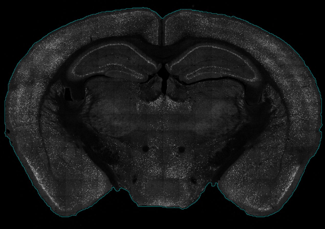

3.2 Registration of a slice

The register() function is one of the generic functions of the package. Because of this, what the function does depends on the type of objects being fed into it. The register() function can be used on both slice and mouse objects. Examples of how to used this function with slice or mouse objects are found under the Usage section.

Pull up the help page with the code below:

?register

If you use a mouse object with the function you need to specify which slice_ID and which hemisphere you want to register, because a mouse object may contain many slices.

Let register our example image using a mouse object! The code below will look for slice 1_4 in mouse_733 and apply the filter settings with the brain.threshold. Note that the mouse object may contain many slices, so that is why we need to specify which slice_ID and which hemisphere to register

mouse_733 <- register(mouse_733, 
                      slice_ID = "1_4",
                      hemisphere = NULL,
                      filter = filter)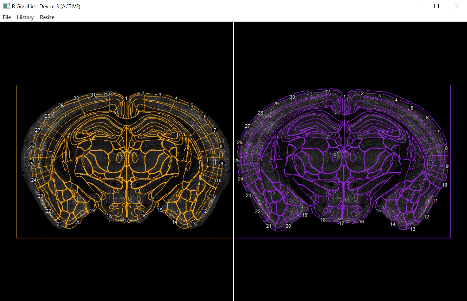

A graphics window should pop up showing the atlas superimposed on the registration image in two outlines. The yellow side is “atlas space” so the correspondence points appear around the boundaries of the atlas. The purple side is “image space” so correspondence points should fit around the contours of the actual brain tissue in the image. One this window has loaded, there should be an interactive console interface allowing for the addition, removal, and changing of these default correspondence points. You can read more about the fitting process in the original wholebrain publication.

At this point, you may find it useful to save all your hard work after perfecting the registration. You can save the mouse object to its output folder with the command below.

save_mouse(mouse_733)

Add the timestamp parameter to save the mouse object with today’s date:

save_mouse(mouse_733, timestamp = TRUE)

I recommend always saving with a timestamp so you never lose more than a day’s worth of work if you accidentally overwrite something.

4 Add segmentation data

4.1 Import raw ImageJ data

The segmentation data from ImageJ is stored into .txt files. We can use the import_segmentation_ij() generic function to import the raw data from ImageJ.

mouse_733 <- import_segmentation_ij(mouse_733,
                                    slice_ID = '1_4',
                                    hemisphere = NULL,
                                    channels = c('eyfp', 'cfos', 'colabel'))

The console output indicating successful importation of segmentation data should look like below:

Imported the following files: 

[1] "M_G_eYFP_733_1_4.txt"
[1] "Q_G_eYFP_733_1_4_eYFP.txt"
Imported the following files: 

[1] "M_C2_cfos_733_1_4.txt"
[1] "Q_C2_cfos_733_1_4_cfos.txt"
[1] "733_1_4cfos_SpotSegmentation_ColocOnly.txt"
[1] "M_733_1_4_Fast_G_eYFP_LabelImage_C1_16bit.txt"

Note that currently, this importation function relies on the output of the txt files output from the macros used to segment cells. The macros automatically name the segmentation output txt files for each channel and this import function recognizes the names of the txt files. Since we often stain for eyfp and cfos, and their colocalization colabel, these three are hard coded channel names in the pipeline.

However, there is built-in capability to include additional custom channels. The generalized segmentation macro found here will recursively segment the channel specified in a .tiff image. The output segmentation txt files can be imported with import_segmentation_custom(). Check out the function documentation for more information.

4.2 Creating a segmentation object

After importing the raw segmentation data, the data needs to be reformatted to be compatible with the registration information using wholebrain functions. This is simply done using the make_segmentation_object() function:

mouse_733 <- make_segmentation_object(mouse_733,
                                      slice_ID = '1_4',
                                      hemisphere = NULL,
                                      channels = c('eyfp', 'cfos', "colabel"))

5 Mapping cells to atlas space

5.1 Forward warp data to atlas space

We are ready to map our segmentation data onto atlas space! We will forward warp our segmented cells onto atlas space with the map_cells_to_atlas() generic function.


mouse_733 <- map_cells_to_atlas(mouse_733,
                                slice_ID = '1_4',
                                hemisphere = NULL,
                                channels = c('eyfp', 'cfos', "colabel"),
                                clean =  FALSE,
                                display = FALSE)

5.2 Cleaning mapped cell data

For all slices, there may be an automatic list of regions to exclude for each hemisphere. This is automatically set as a slice attribute when you create it and you can edit it like any other slice attribute as demonstrated earlier. In the slice attributes, a list of these regions can be accessed with $left_regions_excluded and $right_regions_excluded.

When you run the exclude_anatomy function, it will automatically omit the regions for each hemisphere in these lists. The commands below prints the default excluded regions for the left and right hemispheres.

# Print the default regions excluded list for the right hemisphere
print(attr(mouse_733$slices$`1_4`, "info")$right_regions_excluded)

# Print the default regions excluded list for the left hemisphere
print(attr(mouse_733$slices$`1_4`, "info")$left_regions_excluded)

You can directly edit this list as an attribute to add additional regions to omit per hemisphere for each slice object. You simply need to add the region acronym from the Allen Mouse Brain Atlas Ontology. In the example below, we will pretend there was a rip in the primary somatosensory cortex on the right hemisphere and will add this as a region to exclude.

# Get default list
right_regions_excluded <- attr(mouse_733$slices$`1_4`, "info")$right_regions_excluded

# Append the primary somatosensory area to the list of regions to exclude 
attr(mouse_733$slices$`1_4`, "info")$right_regions_excluded <- c(right_regions_excluded, "SSp")

Alternatively, you can enter additional regions to exclude directly as an argument into the exclude_anatomy() function. Pull up the help page of exclude_anatomy to understand how to perform the following capabilities:

exclude the contralateral hemisphere for slices with either a ‘right’ or ‘left’ hemisphere attribute. This automatically removes anything registered to the unused hemisphere.
clean up cell counts that map outside of the brain contours
exclude cell counts from layer 1 of the cortex
manually specify additional regions we want to exclude for each hemisphere. Below we exclude the secondary motor area on the left hemisphere

mouse_733 <- exclude_anatomy(mouse_733, 
                             slice_ID = '1_4',
                             hemisphere = NULL,
                             channels = c("eyfp", "cfos", "colabel"),
                             clean = TRUE, 
                             exclude_left_regions = c("MOs"),
                             exclude_right_regions = c("SS"),
                             exclude_layer_1 = TRUE, 
                             exclude_hemisphere = FALSE,
                             plot_filtered = TRUE)

You can visualize the filtered counts when you set the plot_filtered parameter to TRUE. Note however, that sometimes the graphical rendering will flip the left and right sides.

6 Normalize cell counts by region

Getting cell counts per region normalized by volume or area in mm³ or mm² respectively.

6.1 Get slice volumes

In order to get cell counts per region in each mouse normalized by volume, the exact volume of each region in each slice needs to be calculated. This is accomplished with the function get_registered_volumes(). The function will automatically calculate region volumes per hemisphere for each slice.


# Calculate region volumes for the full slice
mouse_733 <- get_registered_volumes(mouse_733,
                                    slice_ID = "1_4",
                                    hemisphere = NULL)

6.2 Get a combined cell data table

The get_cell_table() function will aggregate all forward warped cell counts across all slices into one data frame named cell_table. This can be especially useful for plotting purposes.


mouse_733 <- get_cell_table(mouse_733, channels = c("cfos", "eyfp", "colabel"))

You can access the cell table for each channel with the $ operator (e.g. mouse_325$cell_table$cfos). We can use this aggregated dataset if we want to plot an interactive “glass brain” plot of all slices in the mouse.

# Plot an interactive 3D plot of the cfos channel
SMART::glassbrain2(mouse_733$cell_table$cfos, jitter = TRUE)

This is a useful function to show an interactive representation of all the cells cells mapped in a single animal.

6.3 Get normalized cell counts

Once get_registered_volumes() has been run for all the slice objects within a mouse, and the forward warped counts have been combined using get_cell_table(), we can use the function normalize_cell_counts() to get normalized cell counts per volume (mm³) and per area (mm²).

This information is stored as a named element in the mouse called normalized_counts.

Tip: The parameter simplify_regions will further collapse the normalized cell counts by certain keywords (e.g. “layer” or “stratum”). If a region name is detected to have one of these keywords, it will merge counts with its parent structure until there are no more keywords found. This reduces the overwhelming amount of substructures that we can compare and helps simplify our analysis.

mouse_733_0 <- normalize_cell_counts(mouse_733, 
                                   combine_hemispheres = TRUE, 
                                   split_hipp_DV = FALSE,
                                   simplify_regions = TRUE)
# Print preview of normalized counts
head(mouse_733_0$normalized_counts)

6.4 Split hippocampal counts into Dorsal/Ventral counts (Optional)

Sometimes, we want to further subdivide the hippocampus into dorsal and ventral subregions. The wholebrain atlas plates are derived from the Allen Mouse Brain Atlas, which does not intrinsically have dorsal and ventral subdivisions for the hippocampus. Our current strategy is to use an AP coordinate cutoff, where hippocampal counts anterior to this cutoff are considered dorsal and posterior to this cutoff are considered ventral. You can accomplish this by setting the parameters split_hipp_DV = TRUE andDV_split_AP_thresh = -2.7 in the normalize_cell_counts function.



mouse_733 <- normalize_cell_counts(mouse_733, 
                                     combine_hemispheres = TRUE, 
                                     simplify_regions = TRUE,
                                     split_hipp_DV = TRUE,
                                     DV_split_AP_thresh = -2.7)
# Print preview of normalized counts
head(mouse_733$normalized_counts)

7 Aggregating mouse data

7.1 Initializing an experiment object

Once you’ve registered enough mice, you can begin adding them into an experiment object. Creating an experiment object is very similar to the way we created mouse and slice objects with one exception–there are certain experimental attributes that are meant to be autopopulated when we add a mouse object to it and should be left alone during object construction.

For example, if multiple mice are added to an experiment object from three different drug conditions, the experiment object’s attribute drug_groups will consist of the names of the three drugs given. Check the help page to see which experiment attributes are autogenerated. You’ll see that the experiment_name, experimenters, and output_path parameters are the only ones we need to be set manually.

Additionally, know that adding mice to an experiment will keep only the processed neural mapping information, not the individual slice information. This is to ensure that unnecessary computer memory isn’t being used during analysis. Therefore, any changes you want to make to cleaning up or modifying individual slice data should be done at the mouse object level.

# Initialize an experiment object
my_experiment <- experiment(experiment_name = "Learned Helplessness",
                            experimenters = c("MJ", "MyInitials"),
                            output_path = "V:\\Michelle Jin\\path_to_output_folder") #Set this to a location where you want your figures/analysis output to save
 
# Add a mouse to the experiment
my_experiment <- add_mouse(my_experiment, mouse_733)

Just like a mouse object, you can save an experiment object, with or without a timestamp.

save_experiment(my_experiment, timestamp = TRUE)

7.2 Combine cell counts across all the mice in an experiment

Once you’ve added enough mice to perform an analysis, we want to aggregate all the data for each mouse together into one dataframe to perform analysis on.

For now we will load a saved example experiment object named lh that already contains all the mapped mouse object data from our learned helplessness mapping experiment.

# Load the presaved data
load("V:\\Michelle_Jin\\Wholebrain pipeline\\LH_analysis\\learned_helplessness_experiment.RDATA")

# Print the names of the mice stores in the learned helplessness experiment object
print(names(lh$mice))
#>  [1] "829"  "831"  "833"  "9658" "9659" "669"  "732"  "733"  "9716" "9753" "9755"

Aggregating the normalized cell counts across mice into one dataframe is done with the combine_norm_cell_counts() function.

lh <- combine_cell_counts(lh, by = c('groups', "sex", "age"))

by is a special parameter that will allow up to take advantage of the many mouse attributes that we have recorded during creation of a mouse object. It is a vector of the mouse attributes we will use to split our dataset into subgroups for comparison. In the example above, we use the group mouse attributes to compare Shock and Context groups which received inescapable shock and context training, respectively. If there were additional groupings of interest, such as splitting males and females to look at sex differences, you can include the sex attribute into the vector, e.g. c('group', 'sex'). Sometimes, certain attributes like drug may not apply to your experiment, so by should only include the variables that you intend on using for group comparisons during analysis to avoid cluttering your combined dataframe. For consistency in the functions used to filter out subgroups, the values of the attributes will all be converted to strings.

8 Quality checking & saving your data

The quality of the segmentation data may depend on many factors including immunolabelling quality, the sectioning and mounting technique, and performance of the segmentation algorithm. We also want to check for “statistical quality” and ensure that there are enough mice per group within a single brain region to compare. There are a few of functions we can use to check the data which can optionally use to clean our mapped dataset. Additionally, both of them contain log parameter which automatically export to the experiment folder a list of regions removed as a .csv file which don’t meet the quality checks.

8.1 Check for outlier counts

The function find_outlier_counts() will first organize counts into sub analysis groups stratified based on the by parameter. Then the mean cell counts for each analysis group and their standard deviation are calculated. If any regions counts for a mouse exceed greater than n_sd (default = 2) for their analysis group, the region and mouse will be marked as an outlier. If log = TRUE then, the output is stored in a csv file with the file stem region_count_outliers_[channel]. This may be helpful to look back at the raw data and examine whether the segmentation algorithm is doing a good job around these regions for a given mouse.

lh <- find_outlier_counts(lh, by = c('groups', 'sex', 'age'), n_sd = 2, remove = TRUE, log = TRUE)

8.2 Checking for the minimum n number

If you want to check that each analysis subgroup has a minimum n represented per brain region, you can use the function enough_mice_per_group(). This function contains by parameter as well. Additionally, This function also automatically keeps only the common regions that are found across all comparison groups.

lh <- enough_mice_per_group(lh, by = "group", min_n = 4, remove = TRUE, log = TRUE)
#> # A tibble: 213 x 4
#>     channel group   acronym     n
#>     <chr>   <chr>   <chr>   <int>
#>   1 cfos    Context AD          2
#>   2 cfos    Context AHN         2
#>   3 cfos    Context APN         3
#>   4 cfos    Context AUDpo       3
#>   5 cfos    Context AV          2
#>   6 cfos    Context CLI         3
#>   7 cfos    Context CS          3
#>   8 cfos    Context III         3
#>   9 cfos    Context LM          2
#>  10 cfos    Context MEPO        2
#>  11 cfos    Context MM          3
#>  12 cfos    Context MPN         3
#>  13 cfos    Context MPT         3
#>  14 cfos    Context NB          3
#>  15 cfos    Context NLOT        2
#>  16 cfos    Context NOT         3
#>  17 cfos    Context NPC         3
#>  18 cfos    Context OP          3
#>  19 cfos    Context PA          3
#>  20 cfos    Context PG          3
#>  21 cfos    Context POST        3
#>  22 cfos    Context PPT         2
#>  23 cfos    Context PRE         3
#>  24 cfos    Context PRNr        2
#>  25 cfos    Context PSTN        2
#>  26 cfos    Context RH          3
#>  27 cfos    Context RR          3
#>  28 cfos    Context SCH         2
#>  29 cfos    Context SF          3
#>  30 cfos    Context SMT         3
#>  31 cfos    Context SUM         3
#>  32 cfos    Context TRN         2
#>  33 cfos    Context VAL         3
#>  34 cfos    Context VMH         3
#>  35 cfos    Context vCA2        2
#>  36 cfos    Shock   AD          2
#>  37 cfos    Shock   AHN         2
#>  38 cfos    Shock   AM          2
#>  39 cfos    Shock   AV          2
#>  40 cfos    Shock   FC          2
#>  41 cfos    Shock   FS          2
#>  42 cfos    Shock   GPe         2
#>  43 cfos    Shock   IAD         2
#>  44 cfos    Shock   IAM         2
#>  45 cfos    Shock   IF          2
#>  46 cfos    Shock   LD          2
#>  47 cfos    Shock   LPO         2
#>  48 cfos    Shock   MA          2
#>  49 cfos    Shock   MPT         2
#>  50 cfos    Shock   NPC         2
#>  51 cfos    Shock   OP          2
#>  52 cfos    Shock   PO          2
#>  53 cfos    Shock   POST        2
#>  54 cfos    Shock   PT          2
#>  55 cfos    Shock   PVH         2
#>  56 cfos    Shock   RCH         2
#>  57 cfos    Shock   RH          2
#>  58 cfos    Shock   SBPV        2
#>  59 cfos    Shock   SCH         2
#>  60 cfos    Shock   SF          2
#>  61 cfos    Shock   SFO         2
#>  62 cfos    Shock   SPA         2
#>  63 cfos    Shock   SSp-un      2
#>  64 cfos    Shock   SUM         2
#>  65 cfos    Shock   TRS         2
#>  66 cfos    Shock   VPMpc       2
#>  67 cfos    Shock   vCA2        2
#>  68 eyfp    Context AD          2
#>  69 eyfp    Context APN         3
#>  70 eyfp    Context AUDpo       3
#>  71 eyfp    Context AV          2
#>  72 eyfp    Context CLI         2
#>  73 eyfp    Context CS          3
#>  74 eyfp    Context FS          3
#>  75 eyfp    Context GENv        3
#>  76 eyfp    Context IA          3
#>  77 eyfp    Context IG          2
#>  78 eyfp    Context III         3
#>  79 eyfp    Context IMD         2
#>  80 eyfp    Context LD          2
#>  81 eyfp    Context MA          3
#>  82 eyfp    Context MD          2
#>  83 eyfp    Context MH          3
#>  84 eyfp    Context MM          3
#>  85 eyfp    Context MPN         3
#>  86 eyfp    Context MPT         3
#>  87 eyfp    Context NB          2
#>  88 eyfp    Context NDB         3
#>  89 eyfp    Context NOT         2
#>  90 eyfp    Context NPC         3
#>  91 eyfp    Context OP          2
#>  92 eyfp    Context PA          3
#>  93 eyfp    Context PG          3
#>  94 eyfp    Context POL         2
#>  95 eyfp    Context POST        3
#>  96 eyfp    Context PP          2
#>  97 eyfp    Context PPT         2
#>  98 eyfp    Context PRE         3
#>  99 eyfp    Context PRNr        2
#> 100 eyfp    Context PSTN        2
#> 101 eyfp    Context PT          2
#> 102 eyfp    Context PVT         3
#> 103 eyfp    Context RL          2
#> 104 eyfp    Context RR          3
#> 105 eyfp    Context RT          2
#> 106 eyfp    Context SF          2
#> 107 eyfp    Context SNc         2
#> 108 eyfp    Context SO          2
#> 109 eyfp    Context SPF         3
#> 110 eyfp    Context STN         2
#> 111 eyfp    Context SUM         3
#> 112 eyfp    Context TRN         2
#> 113 eyfp    Context TU          3
#> 114 eyfp    Context VMH         3
#> 115 eyfp    Context VPL         2
#> 116 eyfp    Context VPM         2
#> 117 eyfp    Context vCA2        2
#> 118 eyfp    Shock   AHN         2
#> 119 eyfp    Shock   AV          2
#> 120 eyfp    Shock   FS          2
#> 121 eyfp    Shock   GPe         2
#> 122 eyfp    Shock   IMD         2
#> 123 eyfp    Shock   LPO         2
#> 124 eyfp    Shock   MD          2
#> 125 eyfp    Shock   MG          2
#> 126 eyfp    Shock   MPT         2
#> 127 eyfp    Shock   MS          2
#> 128 eyfp    Shock   NDB         2
#> 129 eyfp    Shock   NPC         2
#> 130 eyfp    Shock   PF          2
#> 131 eyfp    Shock   PMd         2
#> 132 eyfp    Shock   POL         2
#> 133 eyfp    Shock   POST        2
#> 134 eyfp    Shock   PP          2
#> 135 eyfp    Shock   PVH         2
#> 136 eyfp    Shock   RCH         2
#> 137 eyfp    Shock   RE          2
#> 138 eyfp    Shock   RL          2
#> 139 eyfp    Shock   SF          2
#> 140 eyfp    Shock   SFO         2
#> 141 eyfp    Shock   SNc         2
#> 142 eyfp    Shock   SNr         2
#> 143 eyfp    Shock   SO          2
#> 144 eyfp    Shock   SPA         2
#> 145 eyfp    Shock   SSp-un      2
#> 146 eyfp    Shock   SUM         2
#> 147 eyfp    Shock   VAL         2
#> 148 eyfp    Shock   VPM         2
#> 149 eyfp    Shock   vCA2        2
#> 150 colabel Context AAA         3
#> 151 colabel Context APN         2
#> 152 colabel Context ARH         3
#> 153 colabel Context AUDpo       3
#> 154 colabel Context CEA         3
#> 155 colabel Context EW          2
#> 156 colabel Context FC          2
#> 157 colabel Context GENv        3
#> 158 colabel Context LGd         2
#> 159 colabel Context LH          2
#> 160 colabel Context LPO         3
#> 161 colabel Context MA          2
#> 162 colabel Context MG          2
#> 163 colabel Context MH          2
#> 164 colabel Context MM          2
#> 165 colabel Context MPN         2
#> 166 colabel Context MPO         3
#> 167 colabel Context MS          2
#> 168 colabel Context NDB         2
#> 169 colabel Context NOT         2
#> 170 colabel Context NPC         3
#> 171 colabel Context PA          3
#> 172 colabel Context PG          3
#> 173 colabel Context PO          2
#> 174 colabel Context POST        3
#> 175 colabel Context PPT         2
#> 176 colabel Context PRE         2
#> 177 colabel Context PVH         2
#> 178 colabel Context PVT         2
#> 179 colabel Context RN          2
#> 180 colabel Context RR          2
#> 181 colabel Context SCs         3
#> 182 colabel Context SH          2
#> 183 colabel Context SPF         2
#> 184 colabel Context SUM         2
#> 185 colabel Context TR          3
#> 186 colabel Context TRN         2
#> 187 colabel Context TU          2
#> 188 colabel Context VMH         3
#> 189 colabel Context VPM         2
#> 190 colabel Context dCA2        3
#> 191 colabel Context vCA2        2
#> 192 colabel Shock   AHN         2
#> 193 colabel Shock   APN         2
#> 194 colabel Shock   IA          2
#> 195 colabel Shock   IMD         2
#> 196 colabel Shock   MEA         2
#> 197 colabel Shock   MG          2
#> 198 colabel Shock   MRN         2
#> 199 colabel Shock   NPC         2
#> 200 colabel Shock   OT          2
#> 201 colabel Shock   PA          2
#> 202 colabel Shock   PMd         2
#> 203 colabel Shock   POST        2
#> 204 colabel Shock   PVH         2
#> 205 colabel Shock   PVT         2
#> 206 colabel Shock   RE          2
#> 207 colabel Shock   RN          2
#> 208 colabel Shock   SCs         2
#> 209 colabel Shock   SH          2
#> 210 colabel Shock   SI          2
#> 211 colabel Shock   SSp-un      2
#> 212 colabel Shock   VTA         2
#> 213 colabel Shock   vCA2        2

8.3 Saving your experiment

If you would like to save your experiment object, just run the function below!

save_experiment(lh)

If you use the timestamp parameter, the experiment object with automatically save with the date as a way to uniquely timestamp your progress.

save_experiment(lh, timestamp = TRUE)

This concludes the end of the mapping tutorial! Check out section 4. Example analysis notebook to see how we apply the analysis and visualization functions in SMARTR to this dataset.